

Aleksandr Aravkin, IHME, University of Washington, Seattle
Abstract
The COVID-19 pandemic was declared on March 11, 2020. In order to help decision makers and hospitals, IHME launched its public facing tool on March 26th, forecasting deaths and hospital resources for US states, with countries and subnationals from Europe and Canada added throughout April.
In this paper, we describe the mathematical methods and statistical models used to develop the forecasts through the end of April 2020. We focus on (1) functional forms used for epidemic trajectories, (2) the mixed effects model used to link locations, (3) extension to multiple Gaussian atoms, (4) the predictive validity framework for uncertainty, and (5) limitations of the parametric form.
1. Overview
The forecasts for COVID-19 deaths and hospital resources from March 26 through the end of April 2020 assumed that (1) all social distancing measures that are in place would stay in place, and (2) any remaining restrictions will be put in place within 21 days.
The forecasting approach, implemented in the CurveFit program, is based on parametric curves fit to data, with parameters modeled using social distancing covariates. A key post-processing step, fitting linear combinations of parametrized models, is also developed to better track data and still be able to forecast in the long term. Parametric functions were chosen because they are interpretable, able to capture key signals from noisy data, and the parametric assumptions made long-term forecasting feasible and stable.
2. Functional Form and Parametrization
We considered multiple functional forms (sigmoid, cumulative Gaussian density, and asymmetric extensions) to model the death rate of the COVID-19 virus, and several spaces to fit the data. The workhorse function for all the forecasts was the cumulative distribution function for the Gaussian distribution (to model cumulative deaths), which corresponds to a Gaussian (Bell-curve) trajectory for daily deaths. Each location was controlled by three parameters (level, peak timing, and trajectory). We developed a statistical model across locations using a mixed effects generalized linear modeling framework, which enforced non-negativity of level and trajectory parameters, and allowed modeling peak timing as a function of social distancing.
3. Curve Fitting Extension Using Gaussian Atoms
As we saw more and more data across locations, it became clear that while some peaks follow the classic Gaussian shape in daily deaths, many do not. Some peaks were wider, some trajectories asymmetric, and overall there was a fair amount of variation in the shape of the curves we see directly in the data. To balance model flexibility (fitting data) with generalizability (forecasting potential epidemic trajectories), we extended CurveFit to a semi-parametric modeling framework, adding a secondary fit to staggered atoms obtained from the initial fit. This approach fit data better across locations, captured asymmetric behavior in time, and generated requisite forecasts (still assuming social distancing remained in place). An example of the resulting forecasts for the United Kingdom is shown in Figure 1.
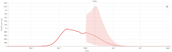
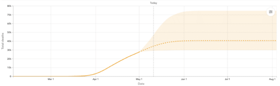
Figure 1: UK Forecasted Daily and Cumulative Deaths, using the CurveFit approach described in Section 2 together with the extension in described Section 3
4. Predictive Validity and Uncertainty
While the initial model (March 26-Aril 5th) used model-based uncertainty quantification (using asymptotic statistics based on curvature information), we developed a new approach relying on out-of-sample predictive validity to estimate uncertainty for forecasts April 5th through May 4th. We tracked model performance out of sample to estimate performance into the future, using this analysis to generate forecast uncertainty. The resulting predictive validity (PV) framework is agnostic to the model or modeling pipeline and was applied to both the initial CurveFit analysis as well as to the extension in Section 3.
The natural quantities to consider when analyzing and generalizing these errors for PV estimation are (1) how many data points we have, and (2) how far out we are forecasting. The models are run repeatedly (as many times as we have data points) to tabulate out-of-sample residuals along these dimensions, and the residuals are used to generate future uncertainty estimates. The residual analysis is depicted in Figure 2, and the analysis is used to inform the uncertainty shown in Figure 1.
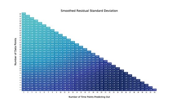
Figure 2: Cross-location predictive validity analysis of out-of-sample residual standard errors incurred by CurveFit. Errors increase with forecast horizon and decrease when we have more data-points to fit the model
5. Limitations
The initial purpose of the CurveFit approach was to estimate timing of peaks to help hospitals plan for surge in equipment need. The assumption on the shape of the epidemic required social distancing to stay in place. In the final sections of the paper, we discuss the limitations and difficulties of using a parametric approach to forecast epidemics under changing conditions, as well as other challenges we encountered.